coderec: Detecting Machine Code in Binary Files
Firmware reverse engineering comes with some unique challenges compared to the reversing of programs that run in the user space of some mainstream operating system. You will encounter one of them before Ghidra’s Code Browser even opens. Let’s illustrate it at a concrete example: I recently got myself some old Cisco devices off eBay as I was curious to have a look at their proprietary IOS operating system. However, when loading the IOS image into Ghidra1 you are greeted with the following screen:
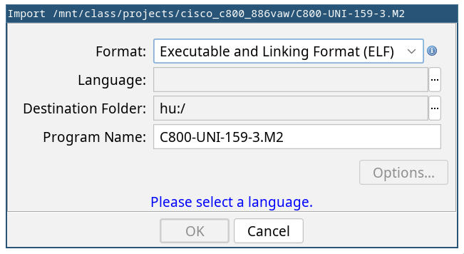
Hm, what’s the processor architecture of this thing2? In this case it’s
pretty easy to figure out the answer by googling the device or having a look at
its PCB. However, in general it is not that simple. To illustrate this let’s
throw unblob at the .firmware section of another IOS image that I pulled
off an older device:
% fd '.*?.bin$'
273704-297420.zip_extract/brisco_fw.uncomp.bin
297420-355662.zip_extract/et2_firmware.uncomp.bin
355664-426609.zip_extract/a.bin
426612-500306.zip_extract/hwic_fpga.bin
500308-618801.zip_extract/vws/dag/CPY-v124_22_t_throttle.V124_22_T5/vob/ios/sys/nms/pse/pse_sm_fpga.bin
618804-671957.zip_extract/vws/dag/CPY-v124_22_t_throttle.V124_22_T5/vob/ios/sys/firmware/pas/hifnhsp/obj/kontrol/flash.bin
671960-870333.zip_extract/vws/dag/CPY-v124_22_t_throttle.V124_22_T5/vob/ios/sys/firmware/pas/hifnhsp/obj/kontrol/hsp.bin
870336-925103.zip_extract/vws/dag/CPY-v124_22_t_throttle.V124_22_T5/vob/ios/sys/firmware/pas/hifnhsp/obj/kontrol/thaddeus_flash.bin
925104-1171822.zip_extract/vws/dag/CPY-v124_22_t_throttle.V124_22_T5/vob/ios/sys/firmware/pas/hifnhsp/obj/kontrol/thaddeus_hsp.bin
Good luck figuring out what processor to select for each of those embedded blobs!
We have a great tool for that purpose, the
Codescanner. It works very well.
However, I have a longstanding
problem
with it. Besides that, it’s written in C++ and Python, and I think that
everything, absolutely everything, should be written in Rust (and open source).
So, let’s write a tool that identifies processor instructions in binary blobs! Or is there anything more fun to do on a sunny weekend?
Note: You can find the source code on GitHub.
Statistics of Machine Code
My core idea for the implementation is based on the
cpu_rec tool by the awesome guys
from Airbus Seclab3.
cpu_rec’s detection mechanism is built around using different n-gram
distributions (bigrams and trigrams) of the instruction bytes as a unique
“fingerprint” of the corresponding processor. It computes these distributions
for a ground truth corpus of code for about 80 different processors, and then
compares them to the distributions of an unknown sample to determine its
architecture.
To better understand how and why this works, let’s have a look at the trigram distributions of code for three popular embedded processors.
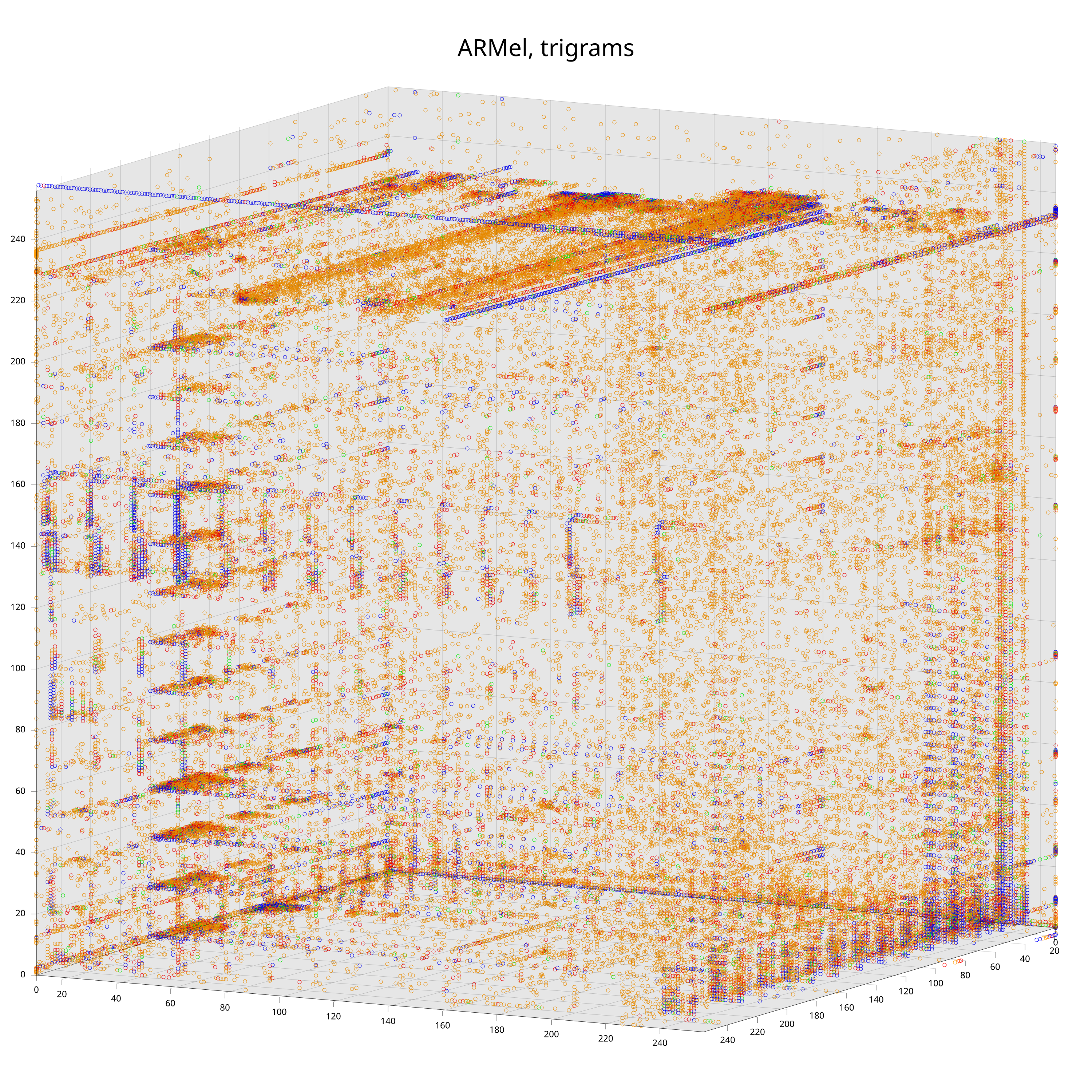
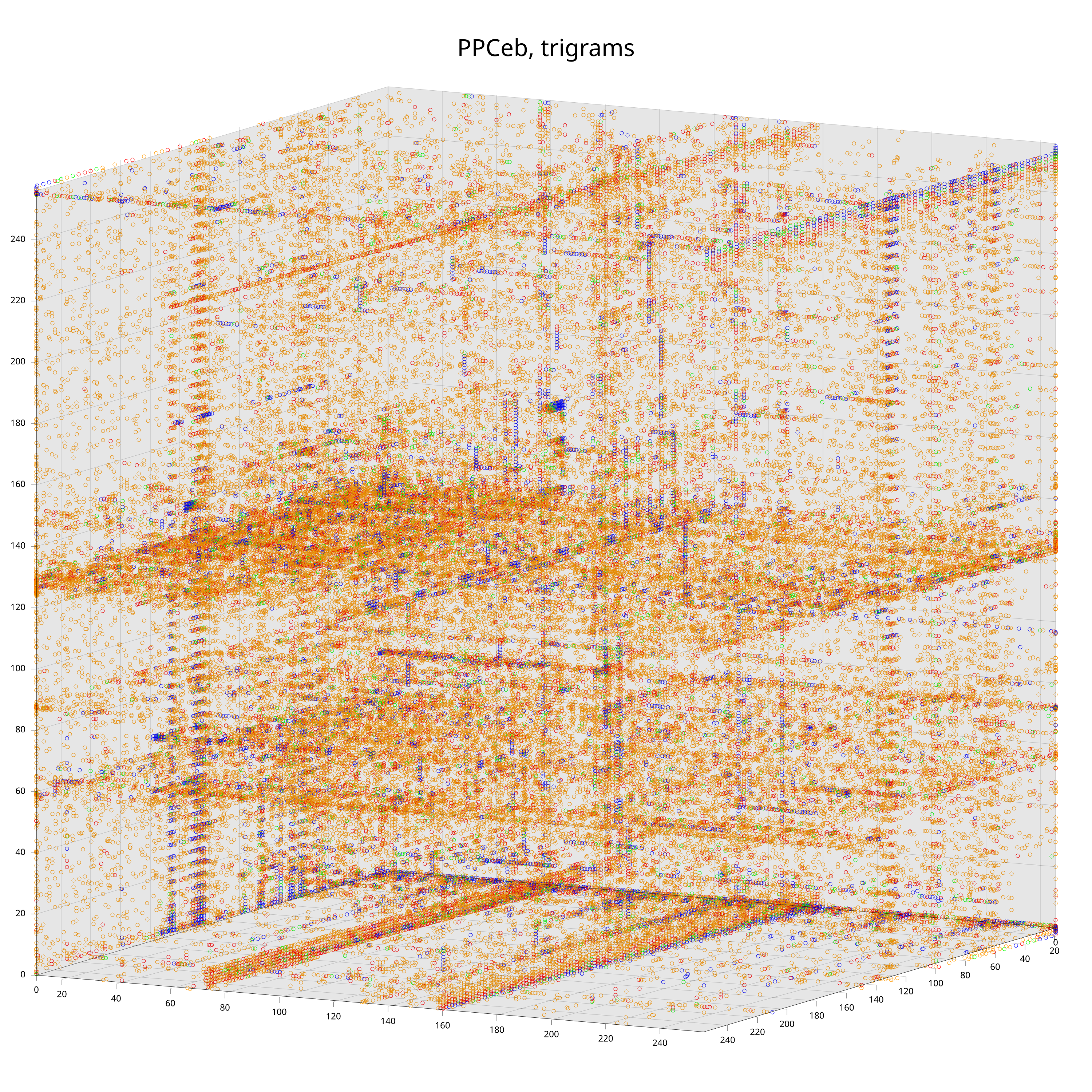
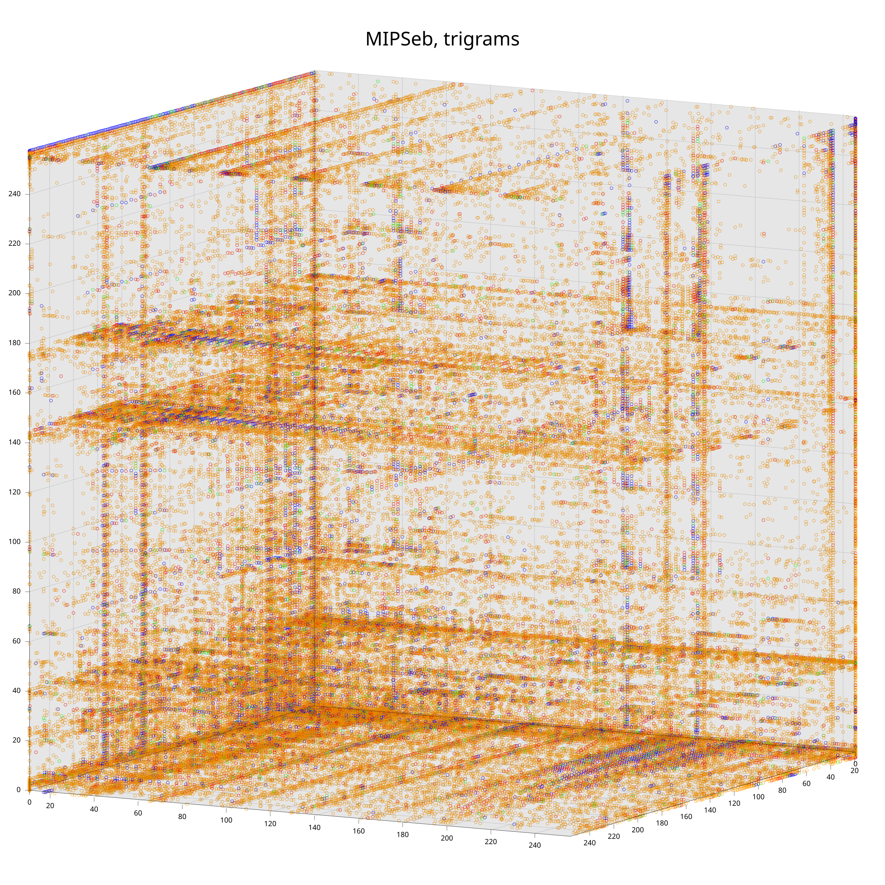
Each data point corresponds to a trigram. The color-coding is according to the probability to observe the trigram (from low to high: grey, orange, red, green, blue). The exact mapping of intervals to colors does not matter here4, what does matter is that one can already see clear differences between the distributions with the bare eye.
I could show similar plots for the bigram distribution, but we would not gain much from that. For bigrams there is a neat different way to interpret them: as conditional probabilities \(P(B | A)\) (given that you just observed byte \(A\), what is the probability that the next byte is \(B\)). We obviously loose some information by doing that transformation, but I still think it’s a good illustration of how much the statistics of machine code depend on the processor.
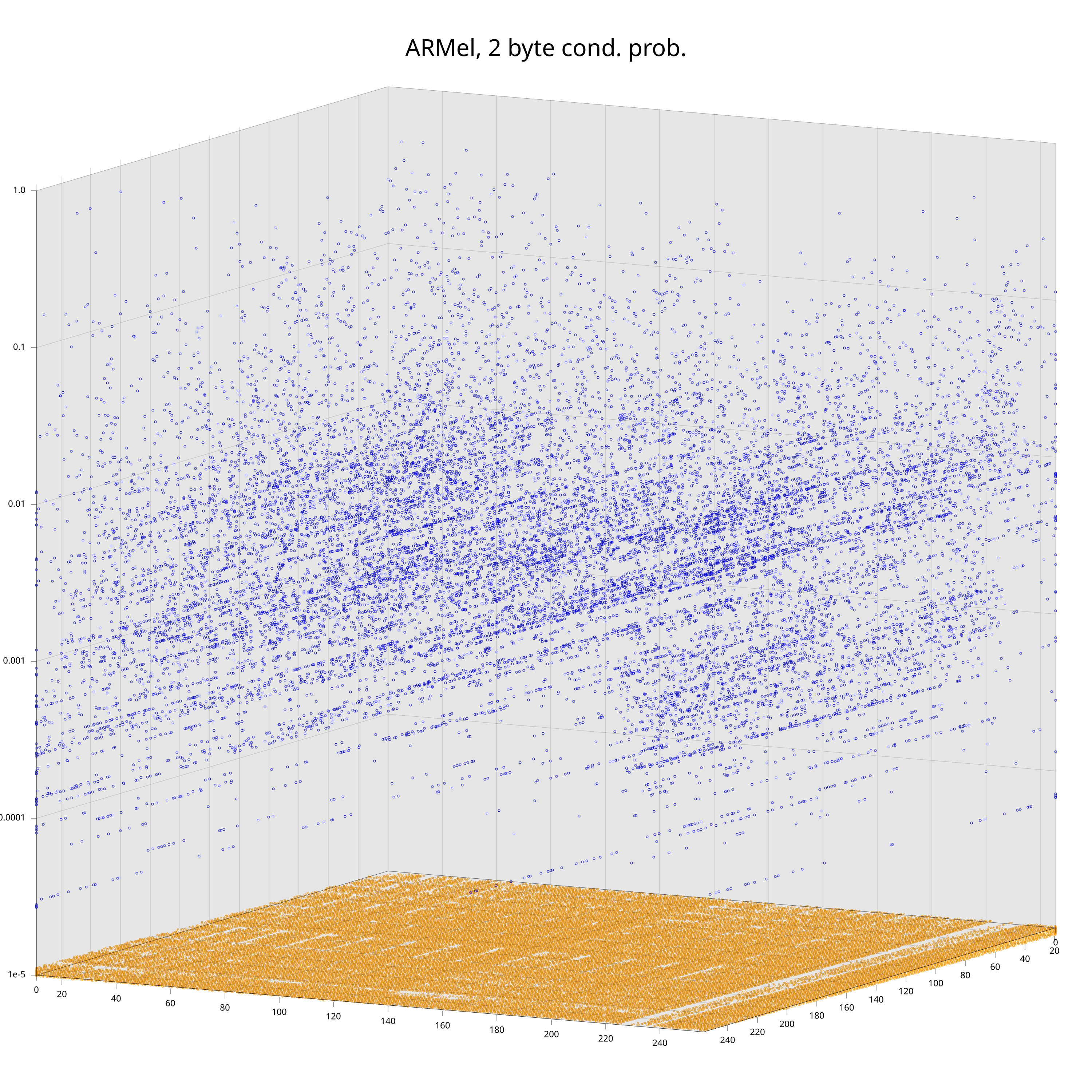
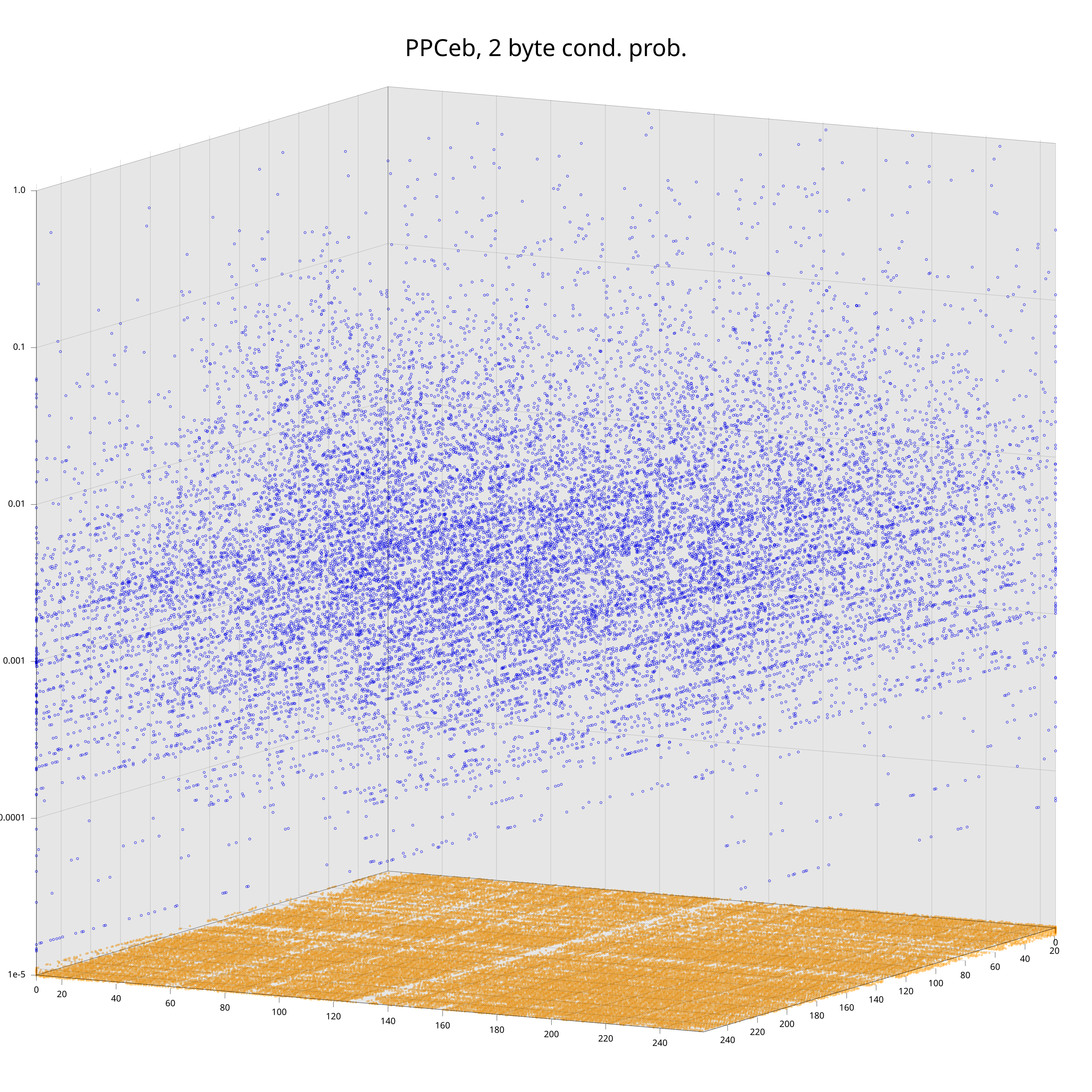
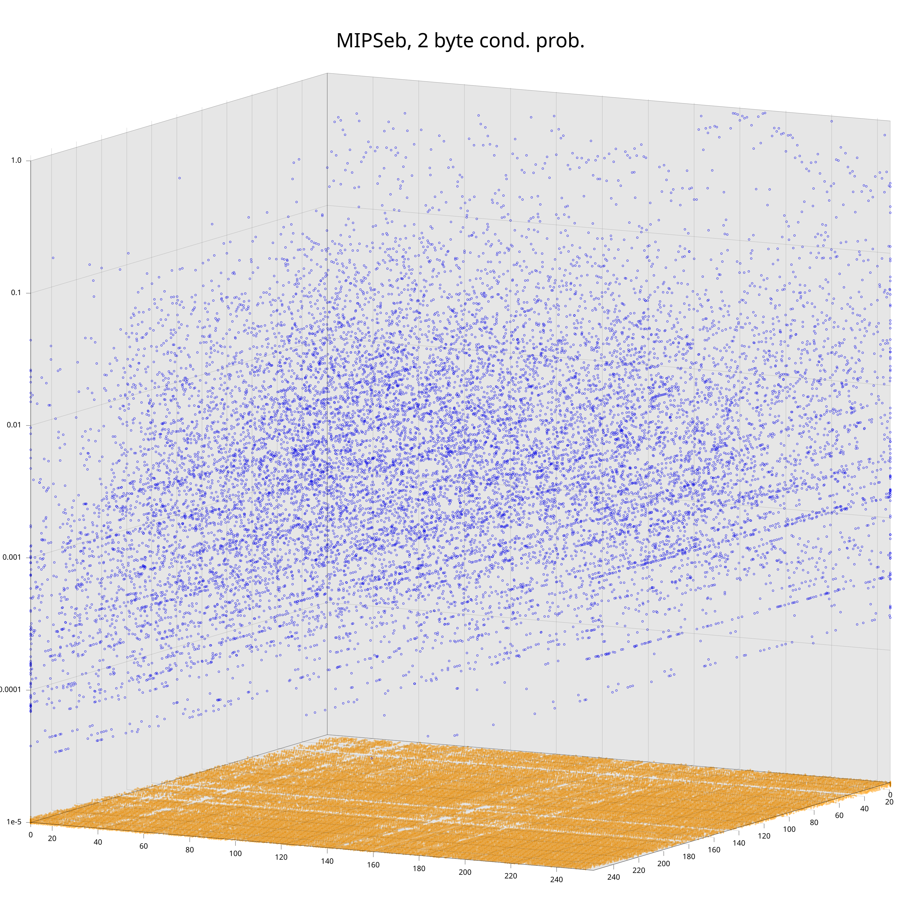
The plots show the conditional probabilities \( P(B | A) \) on the vertical axis, and the projection to the 2d plane at the bottom determines the pair (A, B). Orange points highlight cases where \( P(B | A) = 0 \). While one can vaguely see that the clouds of blue points have distinct features, clear differences are visible in the pattern of orange points at the bottom.
Finding Instructions (and more)
Given the main takeaway of the above section – certain byte-level probability distributions can be used as the “fingerprint” of a processor – all that is really left to do is to slice our target into pieces, compute the relevant distributions for each piece, and find the architecture with the “closest” distribution in the ground truth corpus.
Concerning the choice for distributions (bigrams and trigrams) and
“distance measure”5 (
Kullback-Leibler
divergence (KL), aka. cross-entropy) I decided to stick with cpu_rec’s choices
for now. However, I guess one could experiment with other distributions and
measures as well.
Let’s try this approach (slicing the target into chunks and then computing KL of each chunk with everything in corpus) on two bootroms that I dumped from these Cisco devices I mentioned earlier.
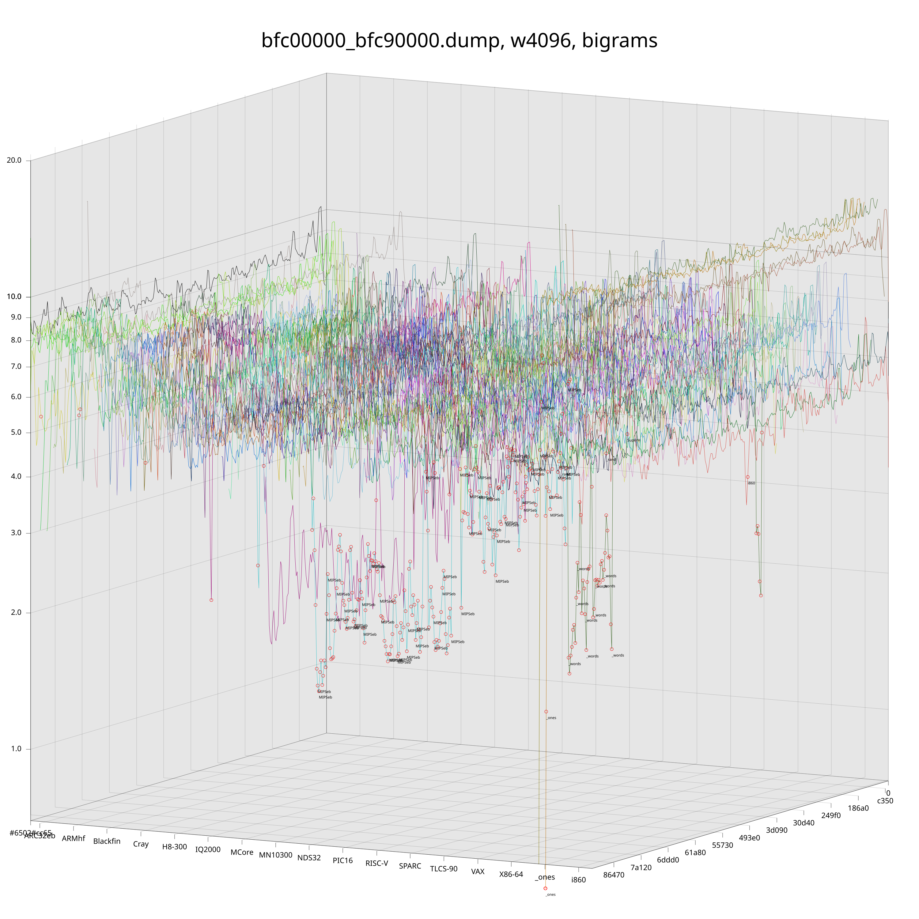
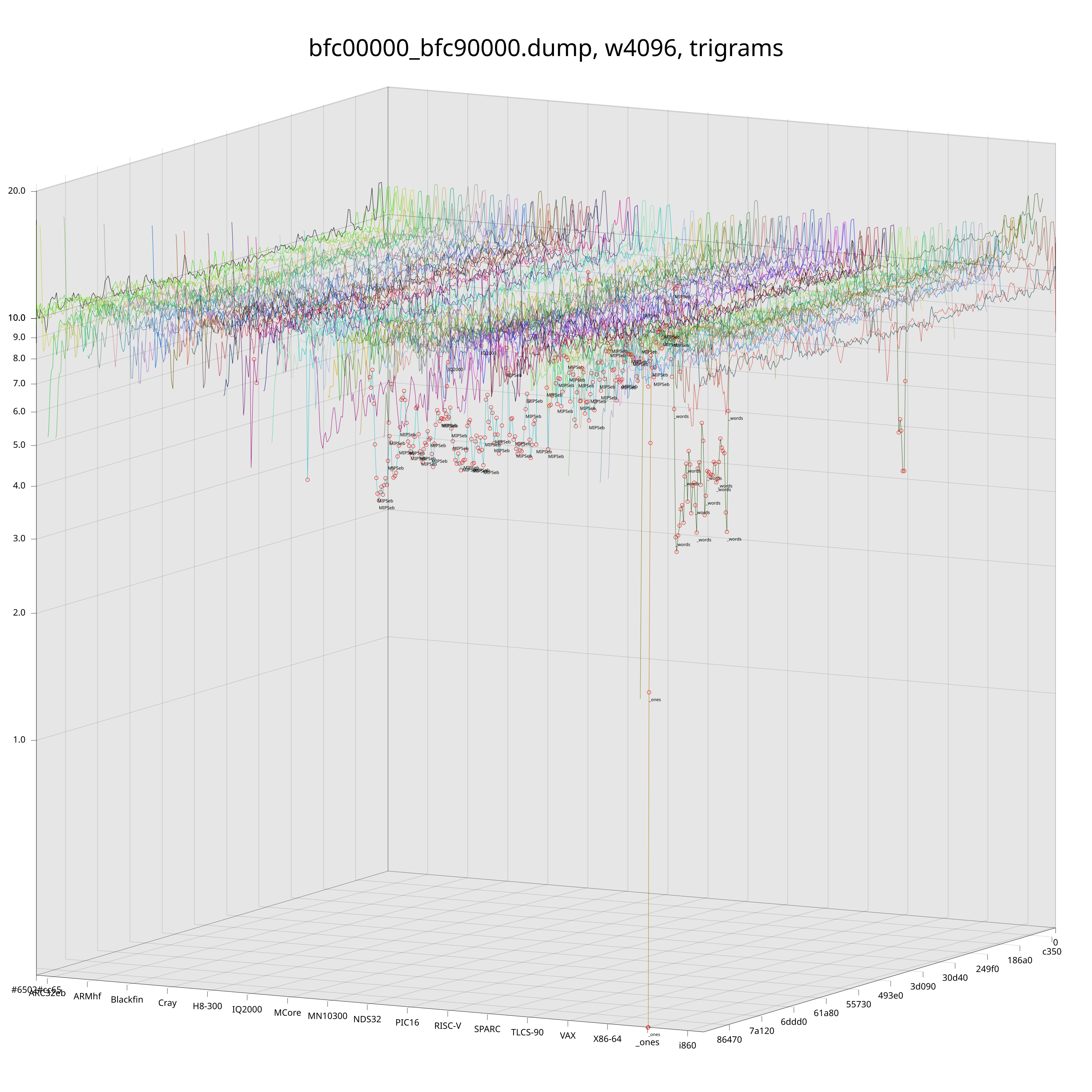
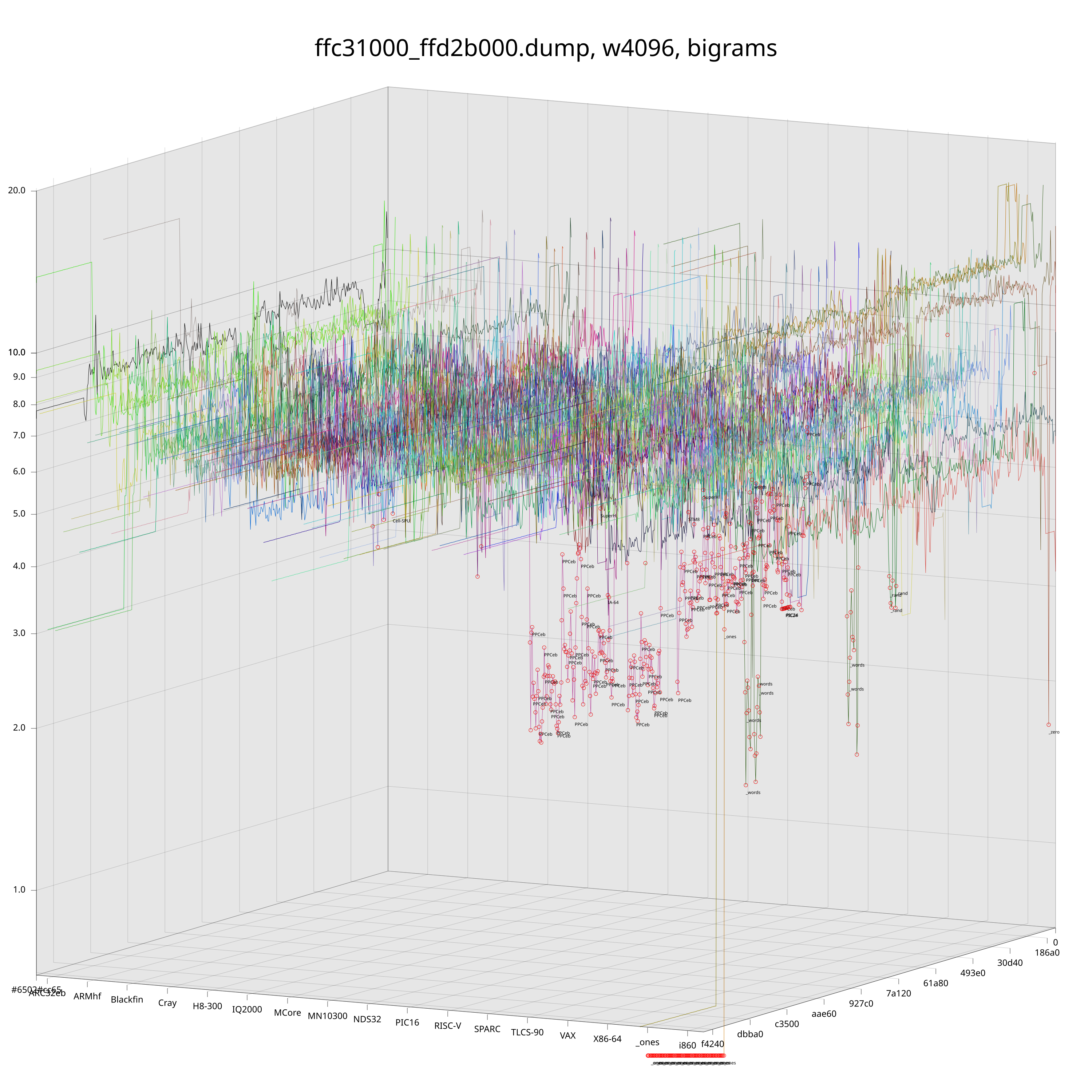
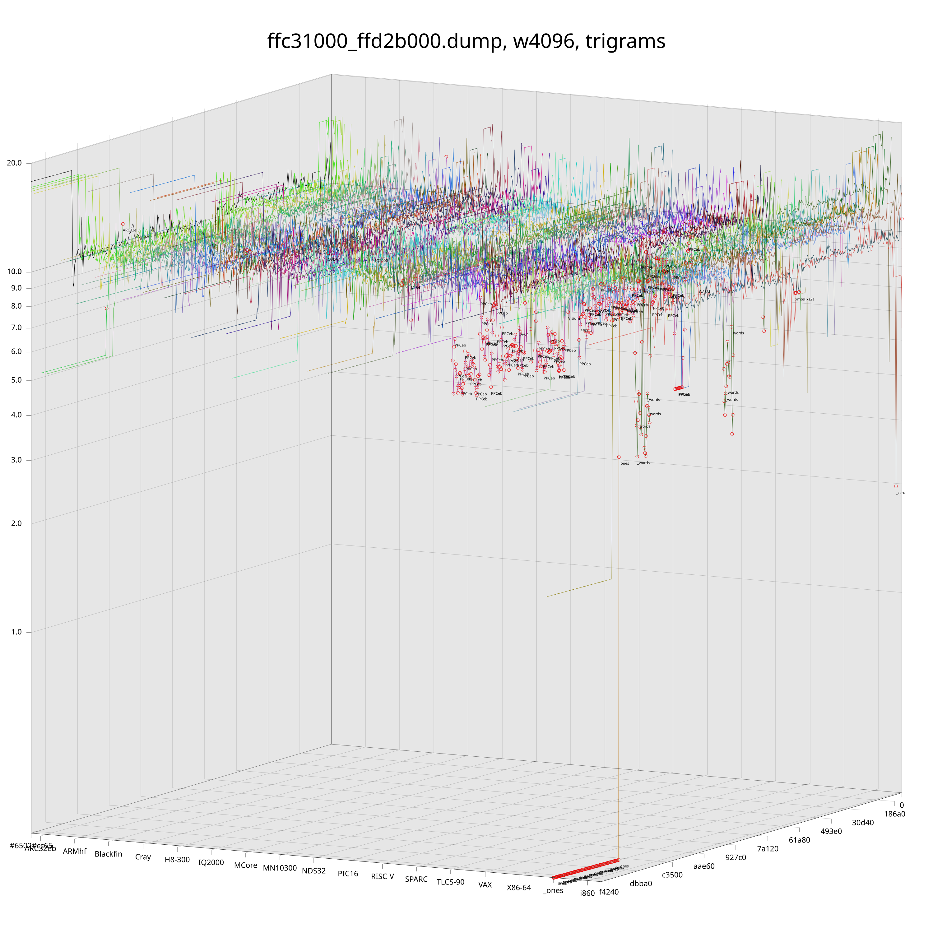
In the above plots, each colored line corresponds to a CPU architecture. These lines “move along” the target file and their z-value is the KL of the arch’s ground truth distribution and the distribution that was observed at the corresponding offset in the target file. Red dots mark the best-fit (lowest) KL for each chunk of the target file and are annotated with the name of the corresponding architecture.
Just by looking at those plots we can already get a pretty good idea of what is going on inside these ROMs. Unfortunately, if we look a bit closer, we will see that the naive detection is still a bit noisy. Fortunately, we still have some tricks up our sleeves that we can pull to reduce the noise level.
Intuitively, there is a difference between an architecture being called because it is “clearly” the closest one for the chunk, or because it is just barely the best fit among many lines that are around the same level.
What we are roughly looking for is something that captures the “statistical significance” of the detection result. My approach for that is currently to calculate the mean and variance of all the KLs in the range. Then, a detection via bigrams or trigrams is immediately significant if it is more than two standard deviations below the respective mean. If both detections are significant but disagree, preference is given to trigrams as I found them to be more reliable. If no detection meets the two-sigma criterion, we still make a call if both detections are lower than the mean minus one standard deviation and agree in their judgement. A final exception is made for the detection of ASCII text, here, a detection via trigrams within one sigma is enough, no matter what bigrams say.
With these additional heuristics in place, we get a relatively clean detection result.


Those are the plots that I find the most useful in practice. There is a 1:1 correspondence between points in the plot and bytes in the file. A point’s x-coordinate is the byte’s file offset, the byte value is used as the y-coordinate, and coloring is used to encode the detection result of the chunk that the byte resides in.
This means we can now leave this tangent that we embarked upon and finally start analyzing this IOS image.

-
After removing one layer of self-extracting archive. ↩
-
Some IOS images are ELF files, however, the
eh_machineentry is complete nonsense. For example, it’s “CDS VISIUMcore processor” for the example from the introduction. ↩ -
They really do a lot of awesome stuff for firmware analysis! ↩
-
What would be quite important are axis labels though … but apparently the best Rust plotting library does not support that. ↩
-
Cross-entropy is not a metric (distance function) in the mathematical sense. ↩